From our previous work with Blackrock (article, paper), we demonstrated that QCML excels in environments where datasets are sparse and imbalanced. This advantage proves particularly valuable in healthcare analytics, where patient data is inherently variable due to individual differences in medical profiles, inconsistent documentation, and the inherent sparsity of medical records. Medical data presents unique challenges:

• Records are often incomplete
• Documentation varies across systems
• Much information exists in unstructured formats like clinical notes
• Privacy concerns limit comprehensive data sharing

These factors make identifying patient similarity particularly challenging, precisely the kind of environment where QCML demonstrates its strengths.

Beyond Standard Accuracy: The Challenge of Imbalanced Datasets

Imbalanced datasets require fundamentally different analytical approaches than balanced ones. Consider our UTI prediction case with data from only 1,436 patients: when 95% of urinalysis results are negative, a model that simply predicts "negative" for every case would achieve 95% accuracy… while providing absolutely no clinical value.

Better Evaluation Metrics for Imbalanced Data

Balanced Accuracy

Balanced accuracy provides a more representative performance metric by giving equal weight to positive and negative classes regardless of their proportions in the dataset:

• TP: True Positive (correctly predicted positive)
• TN: True Negative (correctly predicted negative)
• FP: False Positive (incorrectly predicted positive)
• FN: False Negative (incorrectly predicted negative)

Formula: Balanced Accuracy = (Sensitivity + Specificity)/2

Where:

• Sensitivity = TP/(TP+FN) - Measures the model's ability to correctly identify positive cases
• Specificity = TN/(TN+FP) - Measures the model's ability to correctly identify negative cases

To illustrate this difference, our example "always negative" model would score:

• Standard accuracy: 95% (misleadingly high)
• Balanced accuracy: 50% (0% sensitivity, 100% specificity) - accurately revealing the model's lack of discriminative power

ROC AUC: A Threshold-Independent Metric

ROC AUC (Receiver Operating Characteristic Area Under Curve) evaluates model performance across all possible threshold values by plotting:

• True Positive Rate (Sensitivity) on the y-axis
• False Positive Rate (1-Specificity) on the x-axis

The Area Under Curve provides a comprehensive evaluation metric ranging from 0 to 1:

• 0.5: Indicates no discriminative power (equivalent to random guessing)
• 1.0: Represents a perfect model

ROC AUC is particularly valuable for imbalanced datasets because:

1. It remains insensitive to class distribution, providing reliable performance measurement regardless of class imbalance
2. It evaluates the model's ranking capability rather than just binary decision-making
3. It helps identify optimal prediction thresholds tailored to specific clinical priorities (e.g., minimizing false negatives vs. false positives).

In our UTI example, while a model always predicting "negative" would achieve high standard accuracy (95%), its ROC AUC would correctly reveal its lack of discriminative power (0.5).

Features in Medical Data

When we use the term "feature", we're referring to interpretable properties of input that systems respond to. In medical contexts, features might include patient symptoms, lab values, or demographic information.

Collecting these features from patient data is challenging for several reasons:

• Information may be incomplete or inconsistent
• Some data exists in unstructured formats like notes
• Patient reporting can be subjective
• Documentation varies across healthcare systems
• Privacy concerns limit data sharing

This makes finding patient similarity difficult because the data is inconsistently reported as well as sparse. QCML does well at this kind of dataset.

UTI Prediction Using Patient Similarity

For our investigation of patient similarity in urinalysis data, we utilized the Urinalysis Test Results dataset available on Kaggle.

Establishing the Baseline

We began by creating a classification baseline using standard QCML models. The performance metrics demonstrated promising results:

Model	Balanced Accuracy	ROC AUC
QCML	0.7902	0.765
QCML Weighted	0.7921	0.7668
QCML Ensemble	0.7995	0.8033

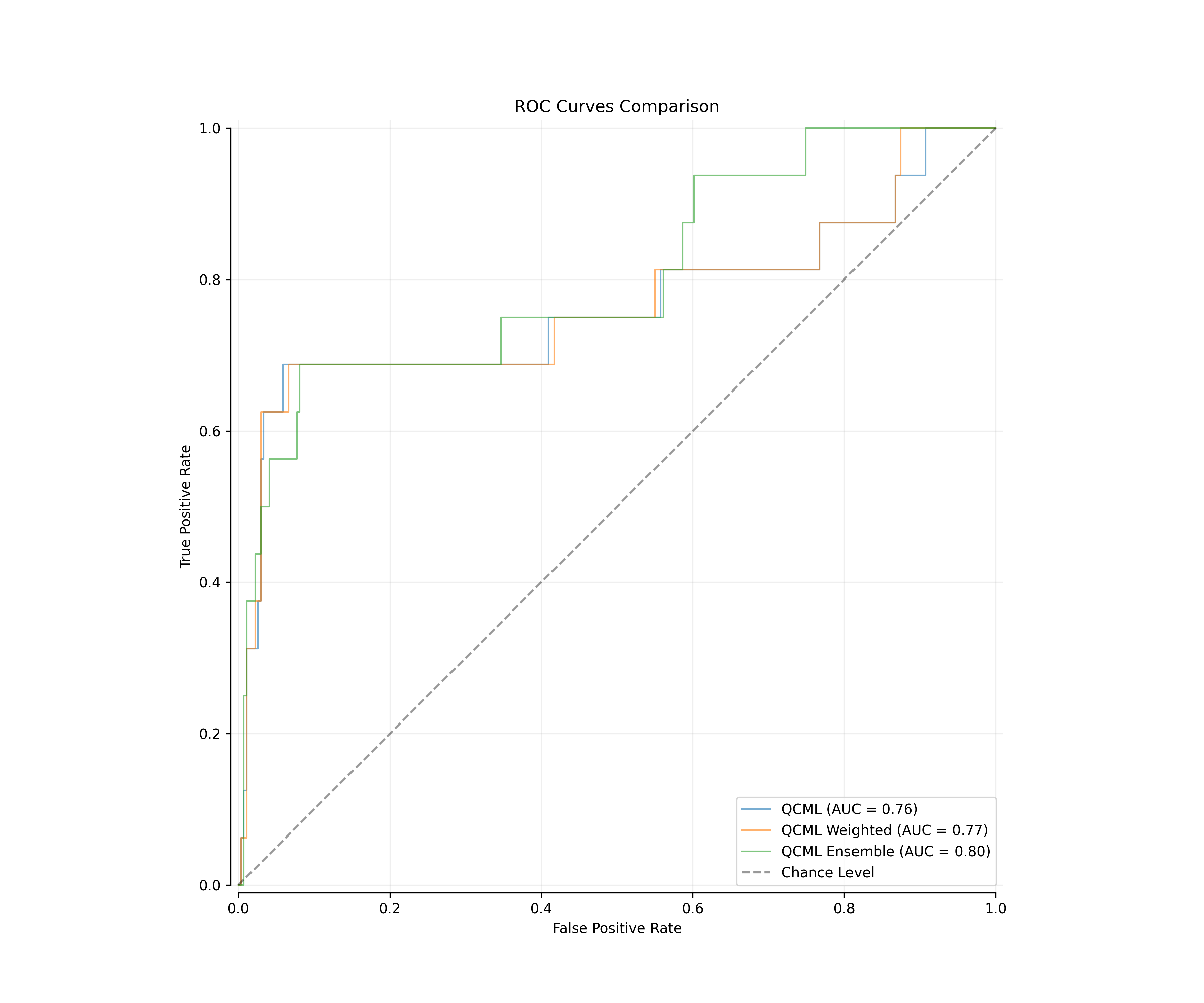
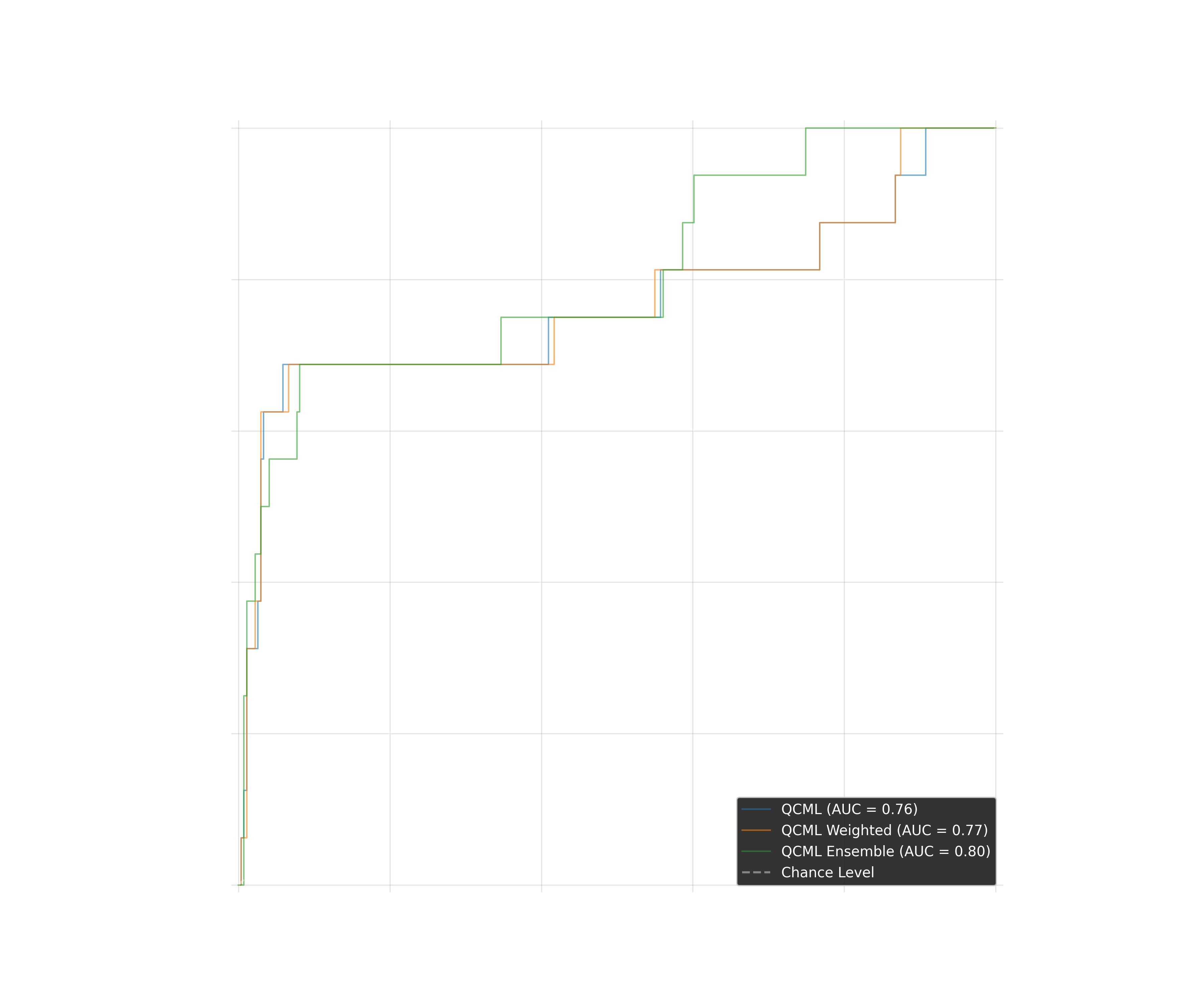
Fig 1: ROC curves comparison showing baseline QCML model performance

Enhancing Prediction with KNN QCML Similarity

Building on the baseline results, we implemented a K-Nearest Neighbors (KNN) using QCML generated similarity matrix. The KNN algorithm works by:

1. Leveraging QCML's superior handling of sparse data to improve similarity calculations
2. Making predictions based on the outcomes (positive or negative UTI results) of those nearest neighbors
3. Identifying the k most similar patient profiles to a new patient record

The visualization of patient distances in our QCML model reveals clear clustering patterns. In the scatter plot, we can observe how positive UTI cases (red points) form distinct clusters, particularly along the top and bottom edges of the distribution, while negative cases (blue points) show more diffuse patterns throughout the feature space. This visual representation confirms that our QCML approach successfully captures meaningful patterns in patient similarity that correlate with UTI outcomes.

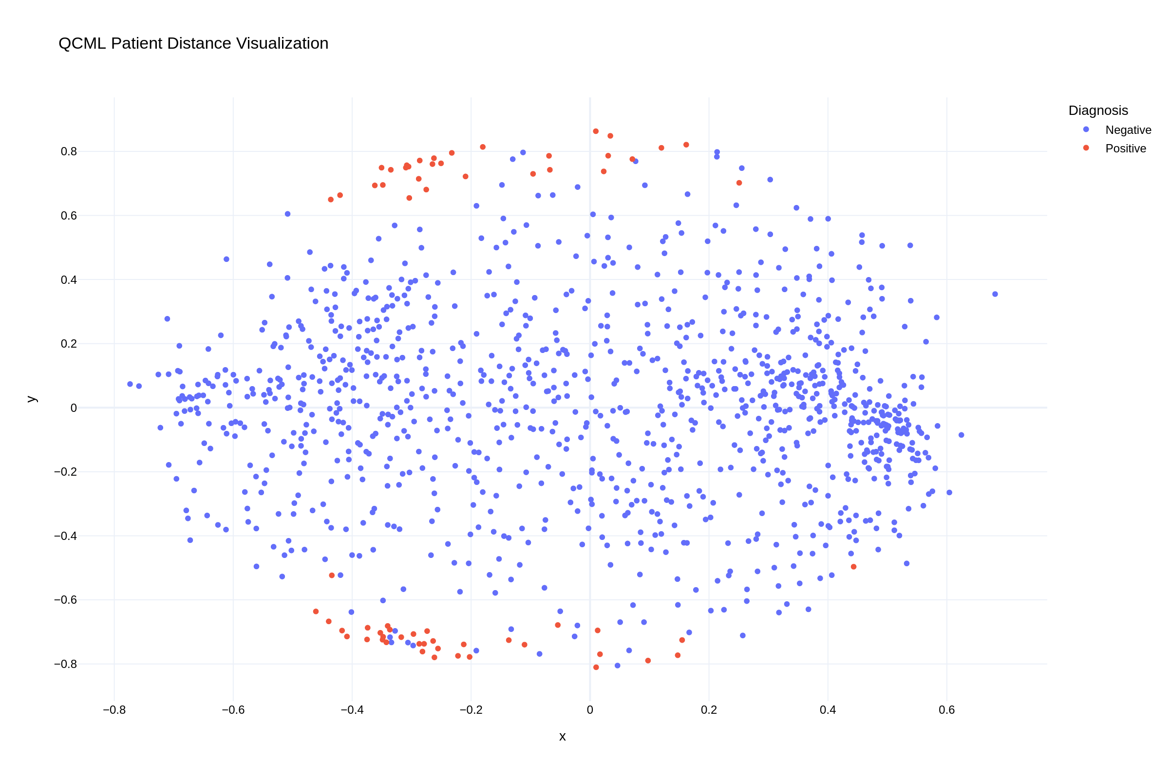
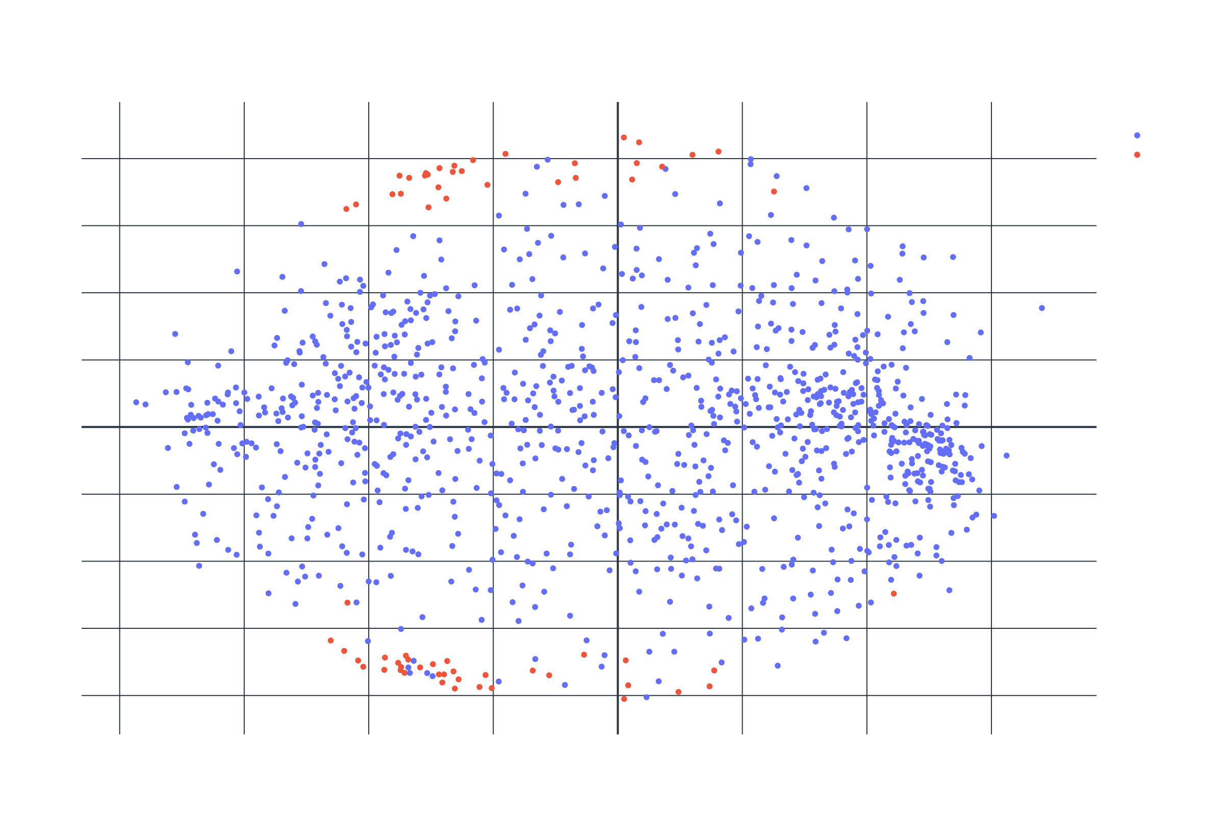
Fig 2: QCML proximity visualization showing patient clustering patterns

Performance Improvements with KNN QCML

When comparing our KNN QCML approach to the baseline models, we observed significant improvements in predictive performance. Fig 3 demonstrates that:

• The KNN QCML model (solid blue line) consistently outperforms the baseline QCML (dashed line)
• Performance stabilizes around k=30 neighbors, achieving an ROC AUC of approximately 0.82
• The confidence interval (blue shaded region) narrows as k increases, indicating robust performance across multiple random seeds

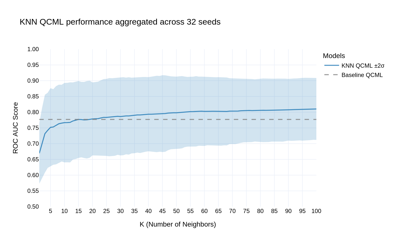
Fig 3: KNN QCML performance aggregated across 32 seeds

Conclusion

Our results demonstrate that QCML is a powerful tool for medical prediction tasks involving sparse, high-dimensional data. Its performance on urinalysis-based UTI prediction highlights its potential for broader clinical applications where data sparsity and class imbalance are persistent challenges. The intuitive clustering of similar patients observed in our visualization has practical significance, as it enables clinicians to understand which patient characteristics drive predictions, enhancing trust and interpretability in AI-assisted medical decision-making.